Courses
Assortment audit

Background
Three times every year assortment audits are carried out to phase in new products and phase out old products. Buyers monitor the old products in the ERP. The data of the new products under review and negotiation are usually incomplete and cannot be loaded into the ERP directly. Therefor you need to create an Excel workbook shared by the Category Managers and Buyers for coordination. You have extracted lists of:
- Categories and responsible Category Managers (data source: ERP).
- Suppliers and responsible Buyers (data source: ERP).
Exercises
Exercise 1 [Data Validation]
Use existing Tables in the Settings Sheet to create drop-down lists:
- Change column Sub category into a drop-down list containing alternatives: All sub categories, “Blank”
- Change column Supplier into a drop-down list containing alternatives: All suppliers, “Blank”
Add additional Tables in the Settings Sheet to create drop-down lists:
- Add a column, to the right of Initial forecast, called Order placed? with a drop-down list containing alternatives: Yes, No
- Add a column, to the right of Deadline delta, called Supply Chain with a drop-down list containing alternatives: Normal, Fragile, Electro static, “Blank”
Exercise 2 [Naming]
- Give all Tables names that describe their contents.
- Give the Sheets names that describe their contents.
Exercise 3 [Conditional Formatting]
Add Basic Conditional Formatting with Scales:
- Lowest value: white.
- Highest value: red.
- Applies to: Supplier price column
Add Custom Conditional Formatting:
- Rule: If cell is empty.
- Fill: red.
- Applies to: Whole Table (Headers excluded).
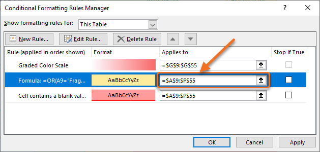
Add Custom Conditional Formatting with Formulas:
- Rule: If cell contains “Fragile”, “Electro static”, “No” or a value less than zero (0).
- Fill: yellow.
- Applies to: Whole Table (Headers excluded).
Exercise 4 [Group, Freeze]
- Freeze columns: Material, Material description, Category manager, Buyer
- Group columns: Sub category to Minimum order quantity
- Group columns: Initial forecast to Supply chain
Exercise 5 [Sliders]
Add Table sliders for:
- Category manager
- Buyer
Format the sliders to fit above the Table.
Exercise 6 [Style and Structure]
Create and apply a new Category Manager cell style:
- Format fill: blue.
- Apply Category manager style to Table columns: Material, Material description, Sub category, Currency, First order, Minimum order quantity, Supplier
Create and apply a new Buyer cell style:
- Format fill: green.
- Apply Buyer style to Table columns: Initial forecast, Order placed?, Delivery date, Supply Chain
Calculation style:
- Apply existing Calculation style to Table columns: Category manager, Buyer, Category, Deadline delta
Color sheet tabs:
- Assortment Sheet: orange.
- Settings Sheet: black.
Exercise 7 [Protection and Security]
- Allow Category Managers to edit Category Manager ranges with password
- Allow Buyers to edit Buyer ranges with password
- Turn on Protect Sheet on all sheets
- Turn on Protect Workbook
- Encrypt the whole Excel document with password
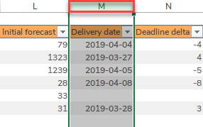
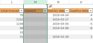
Add columns to the right of other columns:
Step 1 − Select the column to the right.
Step 2 − Right click the selected area and choose Insert.
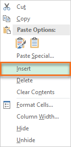
Step 3 − Rename the new column.
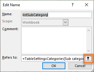
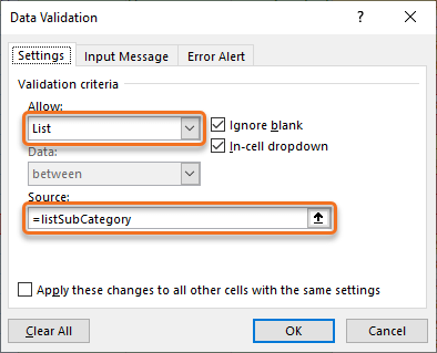
Add drop-down lists:
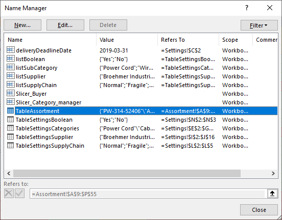
Step 1 − Go to Formulas > Name Manager.
Step 2 − Choose a name.
Step 3 − Select the arrow symbol to change reference. Create a dynamic Structured Reference by selecting the whole list column (without Header).
Step 4 − Go to Data > Data Validation > Data Validation…
Step 5 − Choose List and use the name created in Step 1 – 3 as Source.
Change Table names:
The Name Manager is a helpful tool when changing many names at the same time.
Go to Formulas > Name Manager.
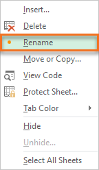
Change Sheet names:
Right-click a sheet tab and select Rename.
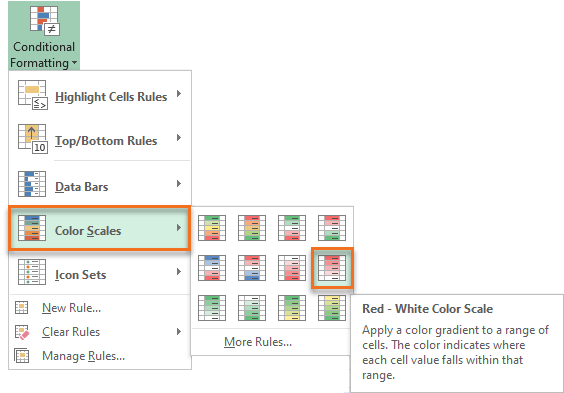
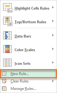
Add Basic Conditional Formatting with Scales:
Go to Home > Conditional Formatting > Color Scales > Red – White Color Scale
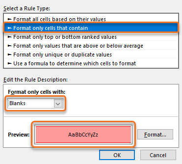
Add Custom Conditional Formatting:
Step 1 − Go to Home > Conditional Formatting > New Rule…
Step 2 − Select:
- Rule Type: Format only cells that contain
- Format only cells with: Blanks
- Format fill: red
Add Custom Conditional Formatting with Formulas:
Step 1 − Go to Home > Conditional Formatting > New Rule…
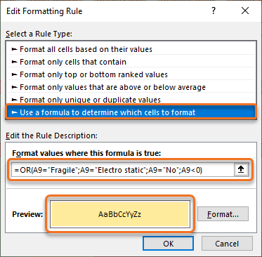
The OR formula is TRUE if any of the 4 conditions are met. Learn more about formulas in the Formulas Module.
=OR(A9="Fragile"; A9="Electro static"; A9="No"; A9<0)
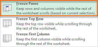
Freeze columns:
Step 1 − Select a whole spreadsheet column to the right of the content you would like to freeze.
Step 2 − Go to View > Freeze Panes > Freeze Panes.
Group columns:
Step 1 − Select the spreadsheet columns you would like to group.
Step 2 − Go to Data > Group.
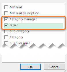
Insert Slicers:
Step 1 − Select the Table.
Step 2 − Go to Design > Insert Slicer.
Step 3 − Select the Slicers you would like to add.
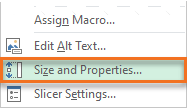
Step 4 − Right-click on a Slicer and select Size and Properties…
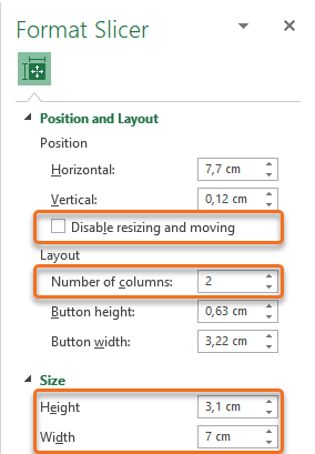
Step 5 − Settings:
- Change: Size
- Adjust: Number of columns
- Last step: Disable resizing and moving
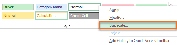
Create a new cell style:
Step 1 − Right-click the Normal style and select Duplicate…
Step 2 − Right-click the new duplicate style and select Modify…
Step 3 − Rename and modify the new style.
Rename sheet tabs:
Right-click the sheet tabs and select Tab Color to choose a color.
Allow Edit Ranges:
Step 1 − Go to Review > Allow Edit Ranges.
Step 2 − Create a new range and choose name, range and password. Repeat password.
Step 3 − Apply.
Protect Workbook and Protect Sheet are also located in the Review menu.
Encrypt the whole document with password:
Go to File > Info > Protect Workbook (drop-down) > Encrypt with Password.
Download solutions file − Case assortment audit solutions
- Category Manager password: gcaW75 (edit specific columns)
- Buyer password: wztX62 (edit specific columns)
- Workbook developer password: bxtF26 (Protect Sheet and Protect Workbook)
- Password to open the document: KwHD53dx
Download solutions file (not password protected) − Case assortment audit solutions unprotected
Tip: Learn Dynamic Formulas
Dynamic formulas with Structured References have been used to further improve the solutions file. Learn more about Structured References and advanced dynamic formulas in the Formulas Module.