Courses
Purchase spend

Background
Management requires an overview report containing Purchase spend per supplier and Sales on supplier level (sales of materials they supply) for last year, 2019. You have extracts containing:
- Purchase orders for last 2 years (data source: ERP).
- Sales orders for last 2 years (data source: ERP).
Exercises
Exercise 1 [Copy Sheet, Remove Duplicates, Naming]
- Create a new Calculation Sheet with a Table containing all the suppliers (do not manually type the supplier names).
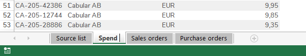
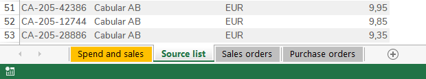
- Name the sheet Spend and sales and name the Table TableSpendSales.
- Color the tab of the Calculation Sheet.
Exercise 2 [SUMIFS, Logical operators, Naming]
Get the total Goods receipt value per supplier for 2019 into the sheet Purchase spend from the sheet Purchase orders. Do not remove any raw data.
Exercise 3 [Number Formats]
Change Number Format of the Purchase spend column to a Custom Number Format:
- Thousands
- Thousands divider: Blank Space ” “
- No decimals
- “K” at the end (kilo, thousands)
Exercise 4 [VLOOKUP, MATCH, SUMIFS, Number Formats]
Get the total Sales order value on supplier level (sales of materials they supply):
- Put the values next to Purchase spend.
- Use the same Number Format as Purchase spend.
Exercise 5 [Conditional Formatting]
Add two different Conditional Formats with Scales:
- Purchase spend: Red color for high values
- Sales: Green color for high values
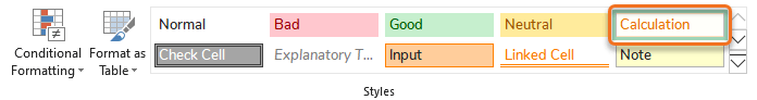
Exercise 6 [Style and structure]
Change cell styles of all formulas in the Data Sheets to the Calculation cell style.
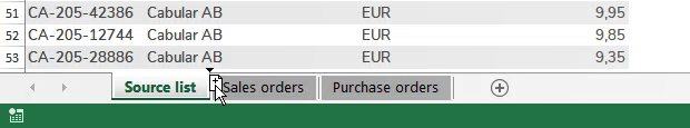
Step 1 − Copy sheet: Hold Ctrl + Left Mouse Button and drag the sheet tab to a new position to create a copy of the sheet.
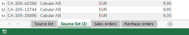
Step 2 − Rename sheet: Left double click on the sheet tab to rename it.
Step 3 − Change sheet color: Right click on the sheet tab to open Tab Color.
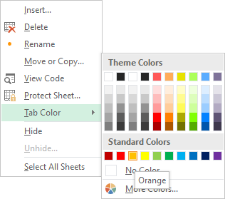
Choose Calculation Sheet colour.
Step 4 − Remove columns: Select redundant columns and remove them by pressing Ctrl + –
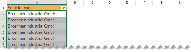
Step 5 − Remove duplicates: Select the whole Supplier name column and go to Data > Remove Duplicates.
Since the data extracts does not only contain data from 2019, multiple criteria must be set not only filtering on suppliers, but also on dates from beginning of 2019 to end of 2019.
To make the formula more dynamic and easier to change if another period should be reviewed, create a Settings Sheet to store the start date and end date.
Name the start date and end date before using them in the formula.
Table: TableSpendSales
Table Header: Purchase spend
= SUMIFS(TablePurchaseOrders[Goods receipt value];
TablePurchaseOrders[Supplier name];[@[Supplier name]];
TablePurchaseOrders[Goods receipt date];">=" & startDate;
TablePurchaseOrders[Goods receipt date];"<=" & endDate
)
Start from one of the existing Number Formats in the Custom category and customize it according to your needs.
Number Format:
# ### K ; -# ### K ; 0There are no Supplier names in the extract Sales orders. This needs to be added from the Source list extract before using SUMIFS.
Table: TableSalesOrders
Table Header: Supplier name
= VLOOKUP([@Material];TableSourceList;
MATCH(TableSourceList[[#Headers];[Supplier name]];TableSourceList[#Headers];0);
0)
Reuse and modify the SUMIFS formula from Purchase spend.
Table: TableSpendSales
Table Header: Sales
= SUMIFS(TableSalesOrders[Sales order value];
TableSalesOrders[Supplier name];[@[Supplier name]];
TableSalesOrders[Sales date];">=" & startDate;
TableSalesOrders[Sales date];"<=" & endDate
)
Use the built-in Conditional Formats with Scales.
Step 1 − Go to Home > Styles.
Step 2 − Select the whole Table column (without Headers) containing formulas.
Step 3 − Select the cell style Calculation.