Courses
Data Validation
Force correct input
Data Validation is used to force a user of the workbook to choose certain predetermined alternatives or value formats when inputting values in the workbook. This is especially useful in order to get good data quality from the start when analyzing with Pivot Tables. For instance you can use limited choices via a drop-down list to force categorization of the data in order to be able to draw conclusions from it. Data Validation is also useful to prevent Pivot Table calculation errors, for instance to prevent a user from entering text into a Table column that should only contain numbers.
Tip: Dynamic Data Validation in Tables
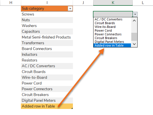
Make sure that the Data Validation is applied to the complete Table data column for the Data Validation to automatically extend to new rows when the Table is extended.
Tip: Naming Referral Shortcut
Press F3 to bring up a list of available names to refer to.
Dynamic drop-down list
The drop-down list (called List in Excel) is a Data Validation criteria forcing the user to choose from certain predetermined alternatives. The list itself is not dynamic in the sense that if you add more alternatives, you have to remember to extend the list range. However, the list can be made dynamic by combining Naming and a Table.
Quick guides
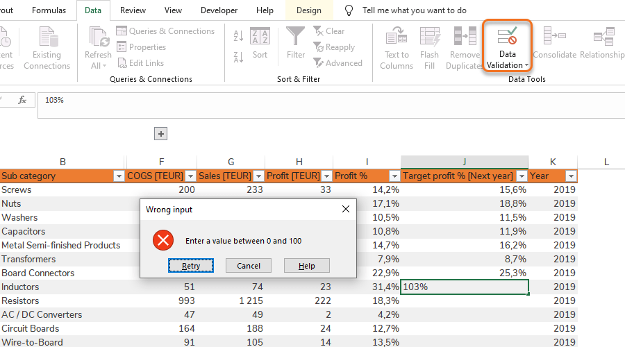
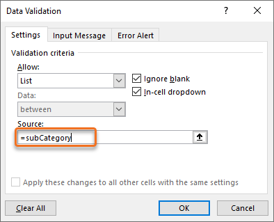
Step 1 – Go to Data Validation > Data Validation…
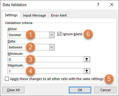
Step 2 – Settings:
Field 1 – Format type to allow
Field 2 – Logical operator
Field 3 – Minimum value
Field 4 – Maximum value
Check box 5 – If for instance only one cell is selected, checking this box will select the other cells with the same setting.
Check box 6 – If this box is unchecked, blank cells will generate error messages.
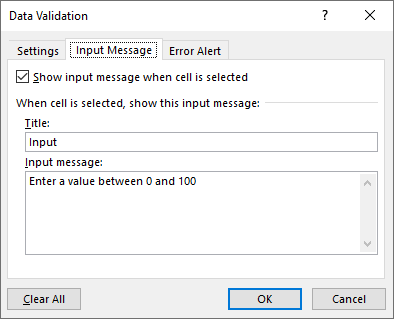
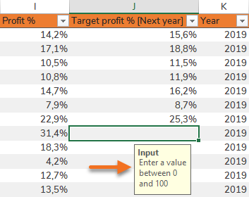
Step 3 [Optional] – Input Message:
Step 4 [Optional] – Choose Error Alert Style:
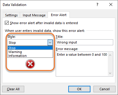
Styles to choose from:
| Error Alert Style: Stop | 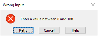 |
| Error Alert Style: Warning | 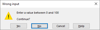 |
| Error Alert Style: Information | 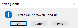 |
Examples of columns where a drop-down list is suitable: Product categories, Demand Planners, Suppliers, Customers etc.
Step 1 [Optional] – Copy preferred column from data extract.
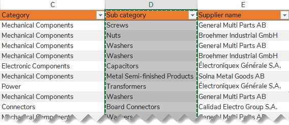
Step 2 [Optional] – Paste into a Settings Sheet.
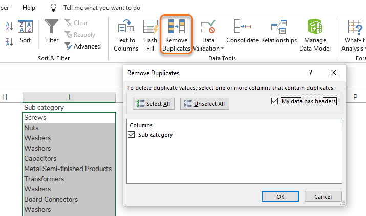
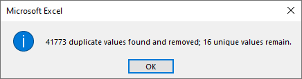
Step 3 [Optional] – Remove Duplicates.
Step 4 – Select the remaining data (including headers) and press Ctrl + T to add a Table.
Step 5 – Select the column (excluding headers) and go to Formulas > Name Manager.
Step 6 – Create a new Name with a Structured Reference to the Table column.
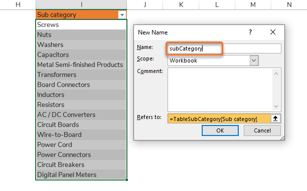
Step 7 – Go to Data Validation > Data Validation… and add a list referring to the Name.
By pressing F3 you get a list of available Names.
Step 8 – Name the cell that the drop-down list is placed in (e.g. subCategoryList) for easy referencing.
Result: When a new row is added in the Table the drop-down list will automatically extend.