Courses
Conditional Formatting
Display of cells
Conditional Formatting uses a similar principle as Number Formats, with the difference that Conditional Formatting changes how a cell is displayed based on the cell value, instead of changing how the cell value itself is displayed. This is an important and dynamic tool to highlight data and make it easier for managers and decision makers to get a quick overview of the data. Conditional Formatting also supports analysis work in a few clicks.
Basic Conditional Formatting
Excel comes with several built-in Conditional Formats that are quite intuitive in their use. The built-in Conditional Formats can be divided into:
- Scales: Single cells are gradually affected by all values in their selected ranges. This means the format of a single cell depends on the other values in the range.
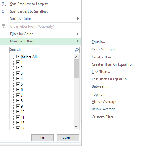
- Limits: Single cells are binarily affected by the limit values. This means the format of a single cell depends only on its own value compared to the manually set limit value.
Tip: Dynamic Conditional Format in Tables
Make sure that the Conditional Format is applied to the complete Table column in order for the Conditional Format to automatically extend to new rows when the Table is extended.
Custom Conditional Formatting
There is also the possibility to create Custom Conditional Formatting rules. These rules can be customized by predefined options, logical statements or formulas. The formats applied to the cells that are triggered by the rules are also customizable.
For Supply Chain purposes we consider the following Custom Conditional Formats to be the most useful:
- Format only cells that contain: The rules are triggered by logical statements.
- Use a formula to determine which cells to format: The rules are triggered by formulas.
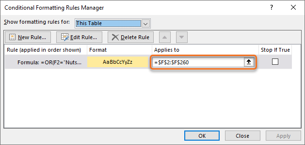
Conditional Formatting Rules Manager
The Conditional Formatting Rules Manager is a handy tool to trace and manage Conditional Formatting in the workbook. The drop-down list in the Manager can be used to filter on Conditional Formatting rules in Sheets and Tables.
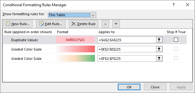
Tip: Use Conditional Formatting Rules Manager
Conditional Formatting can be added, edited and deleted directly in the Conditional Formatting Rules Manager.
Quick guides
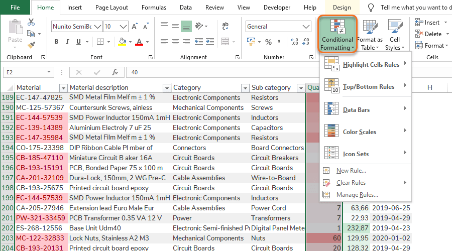
Step 1 – Select a range to format (preferably a complete Table column).
Step 2 – Go to Home > Conditional Formatting.
Step 3 – Hold marker over Bars, Scales or Icons Sets alternatives.
Step 4 – See preview of result in marked cells.
Step 5 – Select preferred Bars, Scales or Icon Sets.
![]()
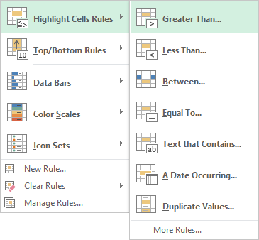
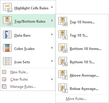
Step 1 – Select a range to format (preferably a complete Table column).
Step 2 – Go to Home > Conditional Formatting.
Step 3 – Select preferred Highlight Cells Rule or Top/Bottom Rule.
Step 4 – Set a limit.
 |
 |
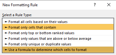
Step 1 – Select a range to format (preferably a complete Table column).
Step 2 – Go to Conditional Formatting > New Rule…
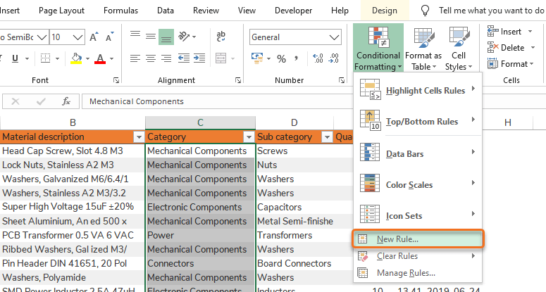
Step 3 – Create a logical statement rule:
Field 1 – Type of rule.
Field 2 – Logical statement.
Field 3 – Value to run the logical statement against.
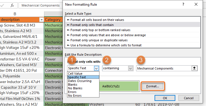
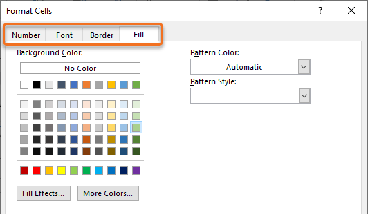
Step 4 – Choose Cell Format (multiple options) for when logical statement is TRUE by clicking Format…
Option 1 – Number Formats
Option 2 – Font Styles: Regular, Italic, Bold, Bold Italic
Option 3 – Borders
Option 4 – Fill effects
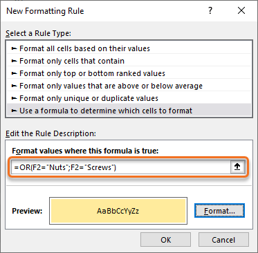
Step 1 – Select a range to format (preferably a complete Table column).
Step 2 – Go to Conditional Formatting > New Rule…
Step 3 – Select Use a formula to determine which cells to format
Step 4 – Write a formula with reference to the first cell in the range.
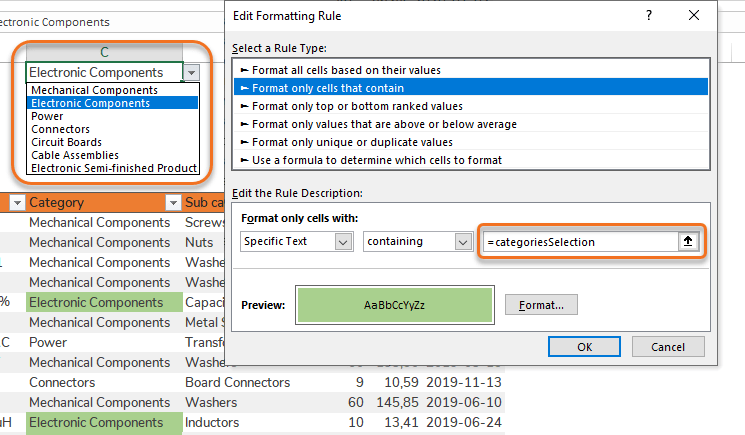
Step 1 – Name the cell that holds the dynamic drop-down list.
Step 2 – Select a range to format (preferably a complete Table column).
Step 3 – Go to Conditional Formatting > New Rule…
Step 3 – Select Format only cells that contain
Step 4 – Write a reference to the named cell. Alternatives selected in the drop-down list will now be formatted.