Courses
Tables
Dynamic workbooks
Using Tables result in dynamic and more standardized Excel workbooks that saves time and lowers the risk of errors in your organization when preparing data for analysis and important business decisions.
Benefits of using Tables
- Structured References: When writing formulas in Tables, Structured References are created. Structured References are easier to understand as they show the actual name of the column header they refer to. Structured References also mean you can resize the Table without changing references to the Table.
- Dynamic data source: When you add additional data right below the last row of a Table, the Table is automatically resized. The Table is also resized if the current data in the Table is pasted over by a larger data set. When adding data to a Table that is used as data source for a Pivot Table, the Pivot Table will take the added data into account. The Table is also well integrated with VBA code.
- Defined elements: The Table has built in features like filters, Slicers and the Totals row that can display sum, average and count etc. The Table also offers easy access to elements like Headers and Totals when creating references.
- Lowers risk of corrupting data: Formulas written in the Table will automatically extend to all the rows, even if the Table is filtered. Sorting the Table will include all the columns, as long as they are defined in the Table. When setting filters without using a Table, a column can easily be excluded by mistake, which means doing a sort will corrupt the data.
- Global style: Global styles can be set for the Table making it easier to keep a coherent design throughout your organization. This will also save time when new workbooks are created since you already have template.
Warning: Empty rows selection
When selecting data there is always a risk that the data set contains empty rows or columns. Make sure you have selected all data rows by pressing Ctrl + ⇧ Shift + ↓ until you have reached the last row of the data set.
Tip: Tables for data interaction
In cases you use the spreadsheet to input and interact with data and not only analyse it, then a Table is a more suitable solution than a Pivot Table.
Table Totals
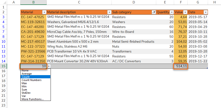
Table Totals is a row at the bottom of the Table. The Totals calculates data column per column and can use several different calculations where the most common are:
- Sum: Calculates the sum of the values in filtered rows.
- Count: Counts the number of filtered rows.
- Average: Calculates the average of the values in filtered rows.
- Min: Finds the min value in filtered rows.
- Max: Finds the max value in filtered rows.
Tip: Control data with Totals
Even if you are not interested in Totals for a certain Table, Totals can be useful as a control row. You may for instance want to set Count to make sure all expected values are accounted for or Sum to make sure percentages sum up to 100 %.
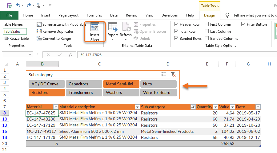
Table Slicers
Slicers make it faster and more convenient to filter data. A Slicer may for instance be set on responsible Category Managers, Product Categories or Suppliers.
It is common to have a Table as a container for raw data, then connecting the Table to a Pivot Table. Slicers are commonly seen with Pivot Tables, but Slicers are also available for Tables.
Quick guides
Step 1 – Select data range including headers by pressing either:
Option 1 – Ctrl + ⇧ Shift + → and then Ctrl + ⇧ Shift + ↓
Option 2 – Ctrl + A
Step 2 – Make sure no data is missing as a result of blank rows or columns.
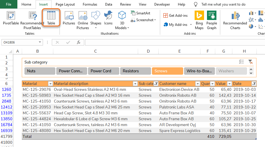
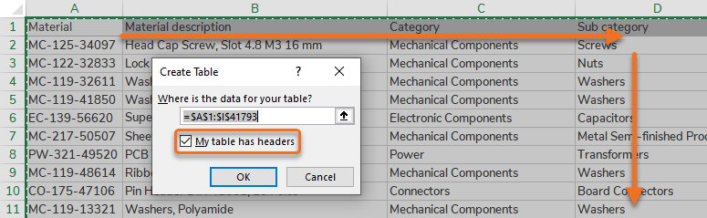
Step 3 – Insert a Table:
Option 1 – Ctrl + T
Option 2 – Go to Insert > Click Table.
Step 4 – Check My table has headers.
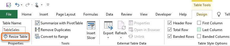
Option 1 – Go to Table Tools > Design (a Table must be selected) > Click Resize Table.
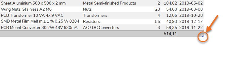
Option 2 – Drag the bottom-right corner to expand the Table.
Option 3 – Add columns to the right of the Table.
Option 4 – Add rows at the bottom of the Table.
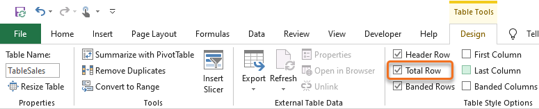
Option 1 – Select a Table then go to Table Tools > Design > Check Total Row box.
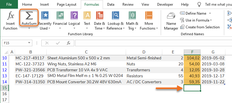
Option 2 – Select a cell right below the Table > Click AutoSum.
Step 1 – Select a Table.
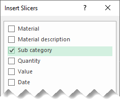
Step 2 – Go to Table Tools > Design > Click Insert Slicer.
Step 3 – Choose Slicers (multiple choices creates multiple Slicers).