Courses
Style and Structure
Coherent design saves time
Design of a workbook, both in terms of style and structure, has a major impact on how easy it is to use and maintain.
When workbooks follow consistent patterns, users spend less time trying to understand how things work. They quickly recognize familiar layouts, naming conventions and formatting choices, which reduces the learning curve for every new file.
A coherent design therefore improves both usability and efficiency. Instead of adapting to a new structure every time, users can focus on the actual task.
Benefits of consistent workbook design
Consistency in workbook design provides several practical benefits:
- Users recognize patterns faster
- Workbooks become easier to maintain
- Errors are easier to detect
- Collaboration becomes smoother
- Development time decreases over time
Even small design decisions such as how inputs, calculations and outputs are organized can have a large impact on clarity.
Recommended standard workbook structure
Recommended workbook structure (sheet tabs) regarding order and coloring:
- Instructions Sheet: The Instructions Sheet should always be first (far left) so it is not missed as it should contain important instructions on how the workbook is built and how it is used.
- Presentation Sheets: The Presentation Sheets contain Dashboards, Pivot Charts, Pivot Tables and in some cases Tables with high level calculations. Not all workbooks contain Presentation Sheets as they are not for presentation purposes.
- Calculation Sheet: The Calculation Sheet (limit to one sheet if possible) contain the main part of the workbooks calculations (the Data Sheets may contain minor calculations). This is where you blend and transform data from the different Data Sheets.
- Settings Sheet: The Settings Sheet should contain all constants, single variables, drop-down list alternatives etc. This way it is easy to change at one single point, just like you expect from any software.
- Data Sheets: Data Sheets are preferably put to the far right as they should not be tampered with apart from some minor calculations that may be necessary. Add additional calculations in Data Sheet to the left of the raw data and mark the calculated columns headers clearly with another color.
Layout and Style levels
Excels dynamic Layout and Styles can be controlled on the following levels:
- Workbook Themes: Themes can control fonts and colors globally for the workbook.
- Table Styles, Pivot Tables Styles and Slicers Styles: Custom Styles can be saved and set as default.
- Pivot Chart Styles and Templates: The predefined styles cannot be customized, only colors can be changed. However, custom templates can be modified and saved.
Workbook Themes
Workbook Themes are a quick way of changing the looks of your workbook.
Tip: Use Workbook Themes
It is recommended to use workbook themes as this means control from one single point in the workbook. If needed, additional styles can be set locally on certain Tables, Pivot Tables and Slicers.
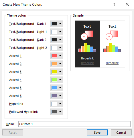
Theme Colors
Theme colors apply to Tables, Pivot Tables, Slicers and Charts.
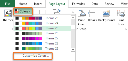
There are many built-in color themes available and there is also the possibility to create custom themes.
Theme Fonts
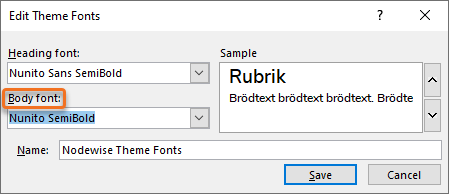
Changing fonts globally from Page Layout is a quick way to style the whole workbook.
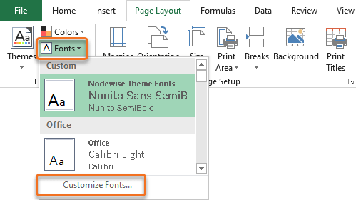
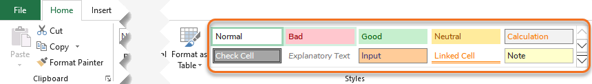
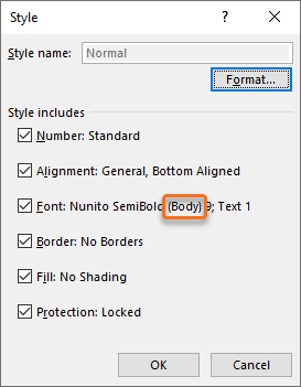
Theme Fonts apply to all the Cell Styles.
Edit for Theme Fonts:
Edit for Cell Styles:
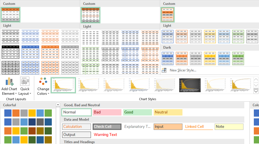
Table, Pivot Table and Slicer Styles
Styles for Tables, Pivot Tables and Slicers are modified in the same way. Their respective options are available when they are selected and the tools menu appears (e.g. Table Tools).
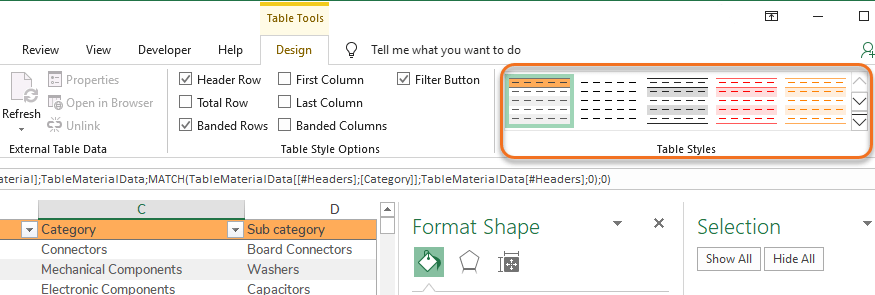
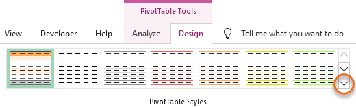
Quick guides
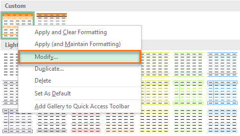
Step 1 – Select a Table, Pivot Table or Slicer.
Step 2 – Go to [Table or Pivot Table or Slicer] Tools > Design > Styles.
Step 3 [Optional] – Extend the drop-down list to view all existing styles.
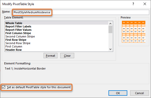
Step 4 – Right-click an existing style > click Duplicate.
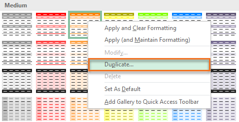
Step 5 – Rename and modify the custom style. It is also recommended that you set the custom style to default for the workbook.
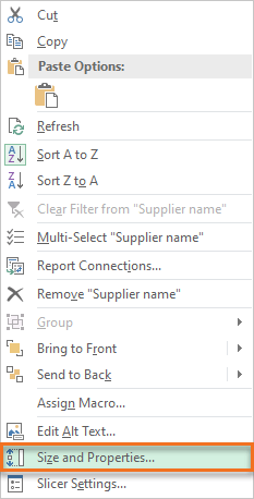
Step 1 – Right-click a Slicer.
Step 2 – Select Size and Properties…
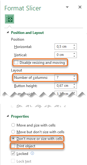
Step 3 – Modify properties in the menu to the right:
- Disable resizing and moving: Recommended to be unchecked (especially for Dashboards), as you want the Slicer to stay fixed.
- Number of columns: Recommended to be set to multiple columns, especially if you want to put the Slicer above a Pivot Table. Most important is that all Slicer items are visible (no scrollbar).
- Don’t move or size with cells: Recommended option so the Slicer stays fixed.
- Print object: If you print Charts to put up on a Lean board for instance, you usually want it to be as clean as possible.
 |
 |
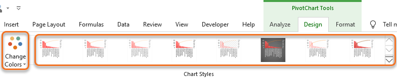
Option 1 – Select a Pivot Chart > Click the Paintbrush.
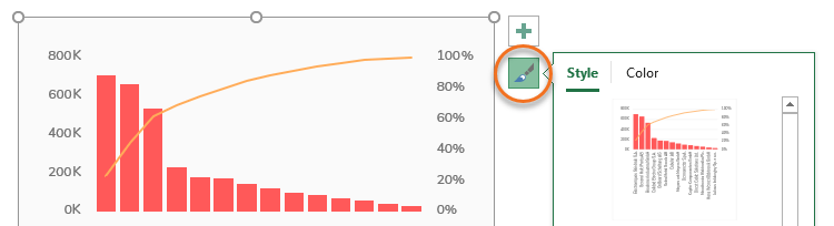
Option 2 – Select a Pivot Chart > Go to PivotChart Tools > Design
Step 1 – Right-click the Pivot Chart that should be used as Template.
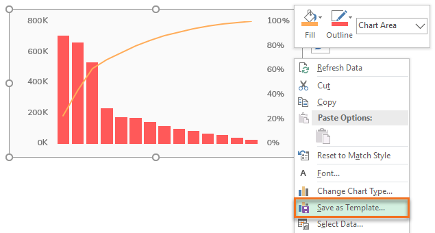
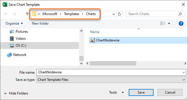
Step 2 – Save the Pivot Chart Template.
Step 1 – Right-click the Pivot Chart to which the Template should apply.
Step 2 – Go to Change Chart Type…
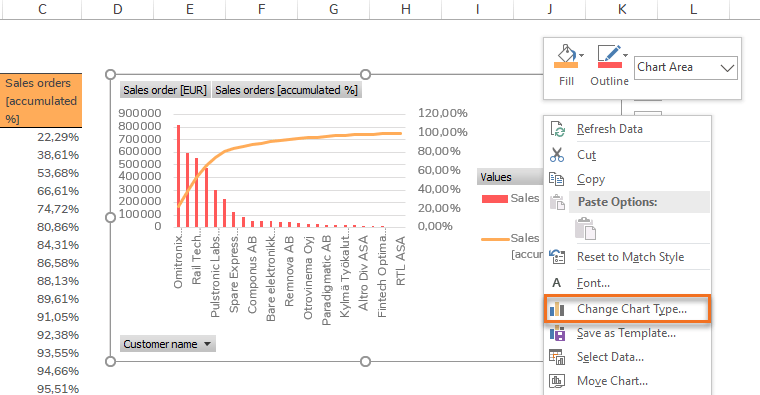
Step 3 – Select the Template.
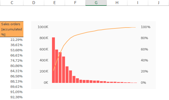
Now the Sales Pivot Chart has been formatted like the Purchase orders Pivot Chart: